Introduction to Mathematica

Mark G. Alford, Washington University Physics Department.

Revised 2020-08-24

This is an introduction to the most basic usage of Mathematica. For more advanced examples, see Mathematica Techniques.

Full documentation is available from The Mathematica website including a Fast Introduction. There are tutorials at Mathematica Resources.

Running Mathematica
There are two ways to use Mathematica: the Notebook interface and the Command-line interface.
- Notebook: Graphical interface. Convenient for quick calculations. You have to type Shift+Return to evaluate an expression.
  However, to develop real programs you will want to create a "Package" file containing Mathematica code. See Mathematica Techniques for instructions on how to do that.
- Command-line: Text-based interface.
  To run it, get a command-line window in the operating system and type
```
math
```
  You may need to type <<JavaGraphics.m to initialize plotting. The command-line interface allows convenient input editing: you can scroll back through previous commands using the up and down arrows, and edit them for re-use. For details see the text-based interface documentation.
Expressions.

In Mathematica, each command you type yields a result. If you terminate the command with a semicolon then the result will discarded and not printed out. This allows you to put several commands on the same line. Much of the notation will be familiar if you know how to program in C or Python.

Comments are enclosed in parentheses with asterisks (* ... *). Comments can be nested.
You can write mathematical expressions using the usual operators:
```
x = 2*(3+4/2)
  10
x^2
  100
y = 2 (3+4/2)   (* you can leave out the multiplication operator *)
  10
1 / 2Pi    (* but be careful to use parentheses where necessary *)
 Pi / 2
1 / (2 Pi)
 1/(2*Pi)
x y        (* same as x*y *)
  100
x=13; y=17; x*y   (* multiple expressions on one line. Only the value of the last expression is "delivered" as the result *)
  221
```
Mathematica treats numbers without decimal points as exact, and does not numerically evaluate them. To force numerical evaluation, use the N function, or put a decimal point in a number somewhere:
```
x = 70/10
  7
x = 70/9    (* No decimal point, so not evaluated *)
  70/9
x = 70.0/9
  7.77778
x = N[70/9]
  7.77778
```
Exponential notation for numbers (e.g. "3.5e15" in C) is done by writing "*^",
```
x = 3.5*^15;
x = 3.5 * 10^15; (* same thing *)
```
To undo assignments and make x and y revert to being symbols of unknown value,
```
Clear[x]; Clear[y];
```

Built-in mathematical functions
These are as you would expect, but they always start with a capital letter, and use square brackets. The constant pi is written Pi, and e is written E.

Sqrt[2]*Cos[Pi]*Exp[-1]
  -Sqrt[2]/E
ArcTan[4]
  ArcTan[4]  (* No decimal points, so not evaluated! *)
ArcTan[4.0]
  1.32582    (* all trig functions are in radians *)
5!       (* factorial *)
  120
Gamma[6] (* gamma function *)
  120

User-defined functions
Let us define a function φ(x) that is shaped like a bump centered at x=0,
```
phi[x_] = 1/(1+x^2);
(* Now try using this function in various ways *)
phi[0.0]
  1.0
phi[1.5]
  0.307692
phi[10.0]
  0.00990099
phi[z]
   (1+z^2)^(-1)
phi[ Sqrt[w] ]
  (1+w)^(-1)
```
We can define a generalized version genphi whose width w must also be specified,
```
genphi[x_,w_] = 1/(1+(x/w)^2);
genphi[0.0,0.2]  
  1.0
genphi[0.8,0.2]  (* now x>>w so the function has a small value *)
  0.0588235
genphi[x,5]
  (1 + x^2/25)^(-1)
```
For serious programming, you will want to create functions that have local variables. This is done using the Module construction. Here is an example, with local variables sx and sy:
```
bump$fn[x_,y_,a_] = Module[{sx,sy},   (* declare local variables sx,sy *)
 sx = x/a;  
 sy = y/a;
 1/(1+sx^2 + sy^2)  (* returned value: don't put a semicolon after it or you'll get "Null"! *)
];
```
You can also exit from the function and return a result res by using Return[res];.
All variables that are internal to the function should be declared as local variables. This avoids accidental conflicts with other functions using internal variables with the same names.
In these examples we defined the function using the = sign which is the immediate evaluation symbol, specifying that the right hand side is to be evaluated immediately. We will see in Mathematica Techniques that for functions that involve numerical calculations one must use the delayed evaluation symbol := which evaluates the right hand side only when the function is called.

Expression manipulation

The Simplify function can simplify complicated expressions. To get good results you may need to give some assumptions about the variables:

Simplify[ Cos[theta] Cos[phi] - Sin[theta] Sin[phi] ]  (* no assumptions needed *)
  Cos[phi + theta]
Simplify[ Sqrt[x^2] * ArcCos[Cos[y]], {x>0,y>0,y<Pi} ] (* assumptions needed *)
  x y

For expressions involving logarithms or trig functions, use FullSimplify which has a more powerful algorithm. It may still need to be told what assumptions to make:

Simplify[ ArcSinh[x] - Log[x + Sqrt[1+x^2]], {x>0} ]
  ArcSinh[x] - Log[ x + Sqrt[1+x^2] ]      (* no luck *)
FullSimplify[ ArcSinh[x] - Log[x + Sqrt[1+x^2]] ]
  ArcSinh[x] - Log[ x + Sqrt[1+x^2] ]      (* no luck *)
FullSimplify[ ArcSinh[x] - Log[x + Sqrt[1+x^2]], {x>0} ]
  0                                        (* at last! *)

Plotting

In the command-line interface you may need to type <<JavaGraphics.m to initialize plotting.
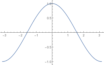
To plot the cosine function, from -π to π,
```
Plot[ Cos[x], {x,-Pi,Pi} ];
```
The plot is itself a "Graphics" object that can be stored in a variable:
```
plot1 = Plot[ Cos[x], {x,-Pi,Pi} ];
```
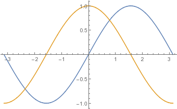
Showing multiple functions on the same plot:
```
Plot[ {Sin[x],Cos[x]}, {x,-Pi,Pi} ];
```
To specify the y-limits of the plot as well as the x-limits, use the PlotRange option:
```
Plot[ Cos[x], {x,-Pi,Pi}, PlotRange->{-0.5,0.5}];
```
To control the positioning of the axes, use the AxesOrigin option:
```
Plot[ Sqrt[1+x^2], {x,-3,3} ];                    (* y-axis begins at y=1 *)
Plot[ Sqrt[1+x^2], {x,-3,3}, AxesOrigin->{0,0} ]; (* Axes cross at (0,0) *)
```
To make the plot window larger on your screen, use the ImageSize option:
```
Plot[ Cos[x], {x,-Pi,Pi}, ImageSize->Scaled[2] ];
```
To write the plot to PDF file, create it as a Graphics object and then "Export" it:
```
plot1 = Plot[ Cos[x], {x,-Pi,Pi} ];
Export["file.pdf",plot1];
```
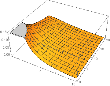
Mathematica infers the format from the dot-extension of the filename. Other possibilities include png, eps, svg, etc.
For a three-dimensional plot, use the Plot3D function,
```
pl3d = Plot3D[ 1/(x^2+y+1), {x,0,10}, {y,0,20} ];
```
Symbolic Integration
For example, to integrate the function 1-x^2 from zero to one:
```
Integrate[ 1-x^2 ,{x,0,1}]
  2/3
```
The limits can be symbols:
```
Integrate[ Cos[x], {x,a,b}]
  -Sin[a] + Sin[b]
```
For a higher-dimensional integral, just give more integration variables along with their limits:
```
Integrate[ Cos[x+y], {x,0,1}, {y,-a,a}] 
  2 Sin[1] Sin[a]
```
Sometimes, in order to get the desired answer you need to give information about the parameters in the form of an "Assumptions" option:
```
Integrate[ r^2*Exp[-r/a],{r,0,Infinity}, Assumptions->{a>0} ]
  2 a^3
```

Numerical Integration

Numerically integrate the function 1-x^2 from zero to one:

NIntegrate[ 1-x^2, {x,0,1}]
  0.666667

or, integrate a user-defined function,

phi[x_] = 1/(1+x^2);
NIntegrate[ phi[x],{x,0,Infinity}]  (* mathematica can integrate to infinity *)
  1.5708

genphi[x_,w_] = 1/(1+(x/w)^2);
NIntegrate[ genphi[x,y],{x,0,Pi},{y,-1,1}] (* two-dimensional numerical integral *)
  1.36271

Complex numbers

The square root of -1 is written is written as I.
```
Exp[I*3.0]
  -0.989992 + 0.14112 I
```
You can obtain real and imaginary parts of any expression using the Re and Im functions. Functions can accept complex arguments, so you can write things like
```
Cos[I*x]
  Cosh[x]
NIntegrate[ Exp[3*I*x] * Exp[-(x-1)^2],{x,-Infinity,Infinity}]
  -0.184946 + 0.0263634 I
```
Complex conjugation is done by the Conjugate function:
```
Conjugate[ 3 + 4 I ]
  3 - 4 I
```
You cannot plot a complex function, but you can plot the real and/or imaginary parts of a complex function:
```
f[x_] = Exp[(-2+3*I)*x];
Plot[ Re[f[x]], {x,0,2}];
Plot[ {Re[f[x]],Im[f[x]]}, {x,0,2}];
```

Arrays and Matrices
A one-dimensional array is a list, which is enclosed in curly braces

v = {2.0, -1.0, 0.0} ;

A matrix or two-dimensional array is a list of lists:

M = {
 {1.3, -2.0, 0.9},
 {-2.2, 0.3, 1.1},
 {-1.4, 1.5, -0.2}
};

Matrix multiplication or dot product uses the dot operator. Scalar multiplication uses "*",

w = 0.5 * M.v
  {2.3, -2.35, -2.15}
w.v
  6.95

There are many useful built-in matrix functions:

Minv = Inverse[M];
MT = Transpose[M];

evals = Eigenvalues[M]
  {2.91742, -1.69075, 0.173336}
evecs = Eigenvectors[M]
  {{-0.512376, 0.661041, 0.548175}, 
   {-0.587781, -0.775991, 0.228806}, 
   {0.397766, 0.553388, 0.731809}}
Tr[M]   (* Note Trace is "Tr", not "Trace" *)
  1.4

You can even take the exponential of a matrix,

Mexp = MatrixExp[M];

Of course, you can calculate the norm of a vector or matrix,

Norm[v]   (* sqrt of sum of absolute value squared of elements *)
  2.23607
Norm[M]
  3.59095

User-defined functions of matrices are just like any other function. Here are some useful ones:

Commutator[a_,b_]    = a.b - b.a;
Anticommutator[a_,b_]= a.b + b.a;
Adjoint[m_] = Transpose[Conjugate[m]];

Subscripting uses double square brackets. Subscripts start at 1. This is one of the differences between Mathematica and C or Python. (The "zeroth" element of a list is its type, actually).

v[[3]]
  0.
M[[2,3]]   (* treat M like a matrix *)
  1.1
M[[2]][[3]] (* treat M like a list of lists *)
  1.1

Printing matrices in a more readable form:

Print[MatrixForm[M]];

Differentiation
Mathematica allows you to use several different notations: "prime", the D[...] function, and the Derivative[...] function.
Function of one variable:

f[x_]=Exp[-x^2];
f'[x]                 (* first derivative, prime notation *)
  -2*x*E^(-x^2)
f''[x]                (* second derivative, prime notation *)
  -2*E^(-x^2) + 4*x^2*E^(-x^2)
D[f[x],{x,5}];        (* fifth derivative, using D function *)
Derivative[5][f][x0]; (* fifth derivative of f, at x=x0 *)

Function of more than one variable:

f[x_,y_] = Exp[-x^2+x*y];
D[ f[x,y], x] (* derivative with respect to x, at fixed y *)
  E^(-x^2 + x*y)*(-2*x + y)
D[ f[x,y], {y,2} ] (* second derivative wrt y, at fixed x *)
  E^(-x^2 + x*y)*x^2
Derivative[5,2][f][x0,y0]; (* fifth deriv wrt x and second deriv wrt y, evaluated at (x0,y0) *)

Series Expansions
Expand Cos[x] around zero, to 4th order:
```
Series[ Cos[x], {x,0,4}]  
  1 - x^2/2 + x^4/24 + O[x]^5
```
Use the Normal function to strip off the + O[x]^5 and get a regular polynomial:
```
Normal[Series[ Cos[x], {x,0,4}]]
  1 - x^2/2 + x^4/24
```
Expand Log[x] around x=1 to 3rd order:
```
Normal[Series[ Log[x], {x,1,3}]]
  -1 + x - (-1 + x)^2/2 + (-1 + x)^3/3
```
The Series function will often produce a simpler answer when you give it some helpful information about the parameters by using the "Assumptions" option:
```
Normal[Series[ Sqrt[ x^2 - a^2 ] , {x,a,1}, Assumptions->{a>0} ]]
  Sqrt[2] Sqrt[a] Sqrt[x-a]
```
Without the assumption that a is real and positive, Mathematica would deliver a much more complicated-looking result.
When expanding around some nonzero value of the argument, another way to get a simpler expression is to rewrite the function in terms of the quantity that you are assuming is small:
```
Normal[Series[ Log[1+epsilon], {epsilon,0,3}]]
  epsilon - epsilon^2/2 + epsilon^3/3
```

Printing numbers
To print numbers and text, just use Print. The SetPrecision function controls the number of digits printed.

Print["The log of ",3.5*^15," is ",Log[3.5*^15] ];
                 15
The log of 3.5 10   is 35.7915
Print["The log of ",3.5*^15," is ",SetPrecision[Log[3.5*^15],8] ];
                 15
The log of 3.5 10   is 35.791539

If you don't like the way exponentials are printed, use the "CForm" function to get the more standard "e" notation:

Print[CForm[3.5*^15]];
  3.5e15
Print[CForm[ SetPrecision[Pi*10^10,5] ]];
  3.1416e10

For more advanced examples, see Mathematica Techniques.